General aspects of the pipeline

%load_ext autoreload

import os 
import sys
import time
import logging
import re
from tqdm import tqdm
import pandas as pd
import numpy as np
import matplotlib.pyplot as plt
from PIL import Image
from natsort import natsorted


sys.path.append(os.path.dirname(os.getcwd()))
from gridgene import get_arrays as ga
from gridgene import contours 
from gridgene import get_masks

sys.path.append(os.path.dirname(os.getcwd()))
from gridgene import get_arrays as ga
from gridgene import contours, get_masks 
from gridgene.mask_properties import MaskAnalysisPipeline, MaskDefinition
from gridgene.binsom import GetBins, GetContour

define the logger : can be None, and is set to INFO

# define the logger :  can be None, and is set to INFO
# Custom logger setup
logger = logging.getLogger('contour_logger')
handler = logging.StreamHandler()
formatter = logging.Formatter('%(asctime)s - %(name)s - %(levelname)s - %(message)s')
handler.setFormatter(formatter)
logger.addHandler(handler)
logger.setLevel(logging.INFO)

Get the files

xenium_path =  '../../xenium_data/HLA/GD_TMA1_S3/fov_filtered'

to_exclude = [
    'TMA1_Selection14_filtered.csv' , # little tumour
    'TMA1_Selection15_filtered.csv', # tonsil
    'TMA1_Selection18_filtered.csv' , # normal
    'TMA1_Selection24_filtered.csv', # tonsl 
    'TMA1_Selection27_filtered.csv', # low quality
    'TMA1_Selection32_filtered.csv', # low quality
    'TMA1_Selection33_filtered.csv', # low quality
             ]
files_tma1 = os.listdir(xenium_path)
files = [os.path.join(xenium_path, file) for file in files_tma1 if file not in to_exclude]
print(len(files))

20

Define Cancer Stroma based on density of genes

This intends to based on defined genes to find tumour areas and empty areas. The stroma/other is defined as the area that is not empty and not tumour.

We need to define:

1. Parameters for tumour contours

   • Genes to consider : Use the marker genes of the gene list with log fold changes for epithelial cells

   • density

   • minimum area

   • kernel size

   this will define for an overlapping area with “kernel size” * “kernel_size” a minimum number of “density” genes of interest. The contiguous area of the contour will have at least “minimum area”

2. Parameters for emptyness contours

   • density

   • minimum area

   • kernel size this will define for an overlapping area with “kernel size” * “kernel_size” a maximum number of “density”/ counts of all genes. The contiguous area of the contour will have at least “minimum area”

# defined with the gene list f
target_tum = ['EPCAM', 'SMIM22','CLDN3', 'KRT18','LGALS4', 'KRT8', 'ELF3','TSPAN8', 'STMN1', 'CD47', 'MYC', 'LGALS3'] 

# param tum
density_th_tum = 25    # 50
min_area_th_tum =  500 #1000     check how much is a cell 
kernel_size_tum = 20   # 20

# param empty
density_th_empty = 20
min_area_th_empty = 50 #400
kernel_size_empty = 10

density_th_tum = 25    # 50
min_area_th_tum = 200
kernel_size_tum = 20   # 20

# param empty
density_th_empty = 20
min_area_th_empty = 400
kernel_size_empty = 10

grab data and derive arrays

file_csv = files[7]
df_total = pd.read_csv(file_csv)
df_total = df_total[['x_location', 'y_location', 'feature_name']]
df_total = df_total.rename(columns={'feature_name': 'target'})
df_total = df_total[~df_total['target'].str.contains('System|egative')]
df_total['X'] = df_total['x_location'] - min(df_total['x_location'])
df_total['Y'] = df_total['y_location'] - min(df_total['y_location'])

n_genes = len(df_total['target'].unique())
height = int(max(df_total['X'])) + 1
width = int(max(df_total['Y'])) + 1

print(f'n genes: {n_genes}')
print(f'shape: {height}, {width}')
print(f'n hits {len(df_total)}')

# this makes the sparse df to an array with the spatial information 
target_dict_total = {target: index for index, target in enumerate(df_total['target'].unique())}
array_total = ga.transform_df_to_array(df = df_total, target_dict=target_dict_total, array_shape = (height, width,len(target_dict_total))).astype(np.int8)

# creating subsets 
df_subset_tum, array_subset_tum, target_indices_subset_tum = ga.get_subset_arrays(df_total, array_total,target_dict_total,
                                                                     target_list=target_tum, target_col = 'target')

n genes: 480
shape: 1809, 1769
n hits 4433228

CTum = contours.ConvolutionContours(array_subset_tum, contour_name='tum')
CTum.get_conv_sum(kernel_size=kernel_size_tum, kernel_shape='square')
CTum.contours_from_sum(density_threshold = density_th_tum,
                       min_area_threshold = min_area_th_tum , directionality = 'higher')

CEmpty = contours.ConvolutionContours(array_total, contour_name='empty')
CEmpty.get_conv_sum(kernel_size=kernel_size_empty, kernel_shape='square')
CEmpty.contours_from_sum(density_threshold = density_th_empty,
                       min_area_threshold = min_area_th_empty, directionality = 'lower') # attention that directionality is lower here 

2025-06-20 15:16:41,914 - gridgen.contours.tum - INFO - Initialized GetContour
2025-06-20 15:16:41,996 - gridgen.contours.tum - INFO - get_conv_sum took 0.0809 seconds
2025-06-20 15:16:42,085 - gridgen.contours.tum - INFO - Number of contours after filtering no counts: 44
2025-06-20 15:16:42,085 - gridgen.contours.tum - INFO - contours_from_sum took 0.0889 seconds
2025-06-20 15:16:42,086 - gridgen.contours.empty - INFO - Initialized GetContour
2025-06-20 15:16:42,758 - gridgen.contours.empty - INFO - get_conv_sum took 0.6722 seconds
2025-06-20 15:16:43,406 - gridgen.contours.empty - INFO - Number of contours after filtering no counts: 20
2025-06-20 15:16:43,406 - gridgen.contours.empty - INFO - contours_from_sum took 0.6472 seconds

Plot contours

fig, axs = plt.subplots(1, 2, figsize=(15, 10))

CTum.plot_conv_sum(cmap='plasma', c_countour='white', ax=axs[0])
axs[0].set_title('Tum points and tum contours')

CEmpty.plot_conv_sum(cmap='plasma', c_countour='white', ax=axs[1])
axs[1].set_title('total points and contours for empty')

plt.show()


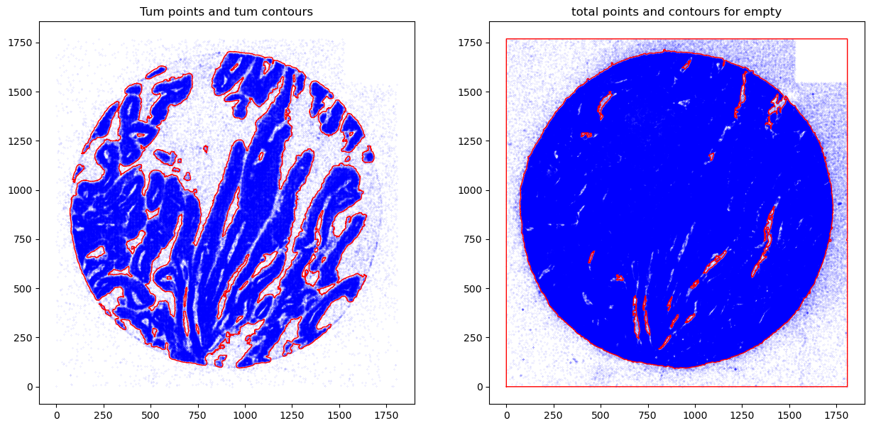
fig, axs = plt.subplots(1, 2, figsize=(15, 7))

CTum.plot_contours_scatter(path=None, show=False, s=0.05, alpha=0.5, linewidth=1,
                           c_points= 'blue',c_contours= 'red', ax=axs[0])
axs[0].set_title('Tum points and tum contours')  

CEmpty.plot_contours_scatter(path=None, show=False, s=0.05, alpha=0.5, linewidth=1,
                               c_points= 'blue',c_contours= 'red', ax=axs[1])
axs[1].set_title('total points and contours for empty')  

plt.show()

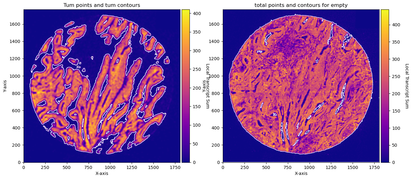
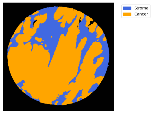
Once you define your parameters of contours you can transform into masks,and obtain, in this case, masks for cancer, stroma and empty areas.
The stroma mask from this analysis is the stroma minus the cancer.

To obtain masks you need to have the contours.

#### obtain masks
GM = get_masks.GetMasks(image_shape = (height, width))

mask_empty = GM.create_mask(CEmpty.contours)
mask_tum = GM.create_mask(CTum.contours)
mask_tum = GM.fill_holes(mask_tum)
mask_stroma = GM.subtract_masks(np.ones((height, width), dtype=np.uint8), mask_tum, mask_empty)          
mask_stroma = GM.filter_binary_mask_by_area(mask_stroma, min_area=700)


GM.plot_masks(masks=[mask_stroma, mask_tum], mask_names=['Stroma', 'Cancer'],
              background_color=(1, 1, 1),
              mask_colors={'Stroma': (65, 105, 225), 'Cancer': (255, 165, 0)},
              figsize = (5,5),
              path=None, show=True, ax=None)

2025-06-20 15:16:45,489 - gridgen.get_masks.GetMasks - INFO - Initialized GetMasks
2025-06-20 15:16:45,516 - gridgen.get_masks.GetMasks - INFO - Subtracted masks from base mask.

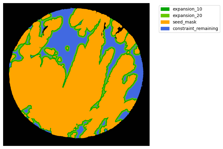
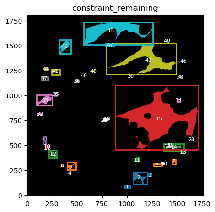
From these we can expand a mask of interest and check their surroundings. In this case we will expand the cancer mask and obtain the interface border masks.

the expansion is given in pixels, so be aware, as in xenium the resolution is approx 1px = 1um so, expansions of 5,10,15,20 would be 5,10,15,20.

TA = get_masks.ConstrainedMaskExpansion(mask_tum, mask_stroma)
TA.expand_mask(expansion_pixels=[10,20], min_area=1000)

# change names and colos«rs! 
mask_colors = {'expansion_10':(0, 165, 0),
               'expansion_20':(100, 200, 0),
               'seed_mask':(255, 165, 0),
               'constraint_remaining':(65, 105, 225) } # Strom}

GM.plot_masks(masks=TA.binary_expansions.values(),
              mask_names=TA.binary_expansions.keys(),
              background_color=(1, 1, 1), mask_colors=mask_colors, path=None, show=True, ax=None,
             figsize=(8, 6))

2025-06-20 15:16:45,792 - gridgen.get_masks.GetMasks - INFO - Initialized GetMasks

Finally we can extract the information from the masks

We have several alternatives here. We can run this analysis: * per object in each mask * per mask, where all the objects of each mask are agglomerated. * per grid. divides each object in a grid size and extracts the information based on this grid. This means the counts are based on objects with same size.

You can get:

* Counts
* Morphological characteristics 

Per mask. run analysis type = ‘bulk’

# 1. Define your masks using MaskDefinition
mask_definitions = [
    MaskDefinition(mask=TA.binary_expansions['constraint_remaining'], mask_name='Stroma_remaining', analysis_type='bulk'),
    MaskDefinition(mask=TA.binary_expansions['seed_mask'], mask_name='Cancer', analysis_type='bulk'),
    MaskDefinition(mask=TA.binary_expansions['expansion_10'], mask_name='CI_10um', analysis_type='bulk'),
    MaskDefinition(mask=TA.binary_expansions['expansion_20'], mask_name='CI_20um', analysis_type='bulk'),
]

# 2. Initialize and run the analysis pipeline
pipeline = MaskAnalysisPipeline(mask_definitions=mask_definitions, 
                                array_counts = array_total,
                        target_dict = target_dict_total,
  )
results = pipeline.run()
df = pipeline.get_results_df()
df

2025-06-20 15:16:46,665 - gridgen.mask_properties.GetMasks - INFO - Initialized MaskAnalysisPipeline with 4 masks.
2025-06-20 15:16:46,666 - gridgen.mask_properties.GetMasks - INFO - Processing mask: Stroma_remaining (bulk)
2025-06-20 15:16:47,099 - gridgen.mask_properties.GetMasks - INFO - Processing mask: Cancer (bulk)
2025-06-20 15:16:47,943 - gridgen.mask_properties.GetMasks - INFO - Processing mask: CI_10um (bulk)
2025-06-20 15:16:48,341 - gridgen.mask_properties.GetMasks - INFO - Processing mask: CI_20um (bulk)

run took 2.0489 seconds

	area	object_id	SPARC	VIM	KRT18	EPCAM	COL4A2	CEACAM1	KRT8	FCER1G	...	TNFRSF18	COL4A5	IL22RA2	IGHA2	CD45RA	IGHD	LST1	VPREB3	mask_name	analysis_type
0	313448	bulk	57272	12381	723	895	4292	151	445	1326	...	1	18	8	6	0	4	1	0	Stroma_remaining	bulk
1	1490024	bulk	58867	23990	183020	240049	7417	34765	59454	6946	...	7	31	64	13	3	11	8	5	Cancer	bulk
2	160338	bulk	28922	7273	1029	1025	3087	127	395	1330	...	1	4	9	0	1	1	1	0	CI_10um	bulk
3	118916	bulk	22367	5109	364	411	2041	66	174	812	...	1	3	7	3	0	0	2	0	CI_20um	bulk

4 rows × 484 columns

Per object in each mask, run analysis type = ‘object’

# 1. Define your masks using MaskDefinition
mask_definitions = [
    MaskDefinition(mask=TA.binary_expansions['constraint_remaining'], mask_name='Stroma_remaining', analysis_type='per_object'),
    MaskDefinition(mask=TA.binary_expansions['seed_mask'], mask_name='Cancer', analysis_type='per_object'),
    MaskDefinition(mask=TA.binary_expansions['expansion_10'], mask_name='CI_10um', analysis_type='per_object'),
    MaskDefinition(mask=TA.binary_expansions['expansion_20'], mask_name='CI_20um', analysis_type='per_object'),
]

# 2. Initialize and run the analysis pipeline
pipeline = MaskAnalysisPipeline(mask_definitions=mask_definitions, 
                                array_counts = array_total,
                        target_dict = target_dict_total,
  )
results = pipeline.run()
df = pipeline.get_results_df()
df

2025-06-20 15:16:48,730 - gridgen.mask_properties.GetMasks - INFO - Initialized MaskAnalysisPipeline with 4 masks.
2025-06-20 15:16:48,731 - gridgen.mask_properties.GetMasks - INFO - Processing mask: Stroma_remaining (per_object)
2025-06-20 15:16:49,625 - gridgen.mask_properties.GetMasks - INFO - Processing mask: Cancer (per_object)
2025-06-20 15:16:51,203 - gridgen.mask_properties.GetMasks - INFO - Processing mask: CI_10um (per_object)
2025-06-20 15:16:51,987 - gridgen.mask_properties.GetMasks - INFO - Processing mask: CI_20um (per_object)

run took 3.8931 seconds

	object_id	area	perimeter	eccentricity	solidity	centroid_y	centroid_x	min_row	min_col	max_row	...	TNFRSF18	COL4A5	IL22RA2	IGHA2	CD45RA	IGHD	LST1	VPREB3	mask_name	analysis_type
0	1	1085.0	169.018290	0.922395	0.847656	85.949309	1004.500461	75	970	102	...	0	0	0	0	0	0	0	0	Stroma_remaining	per_object
1	2	5981.0	503.972655	0.860329	0.536028	178.083264	1118.782812	115	1065	231	...	0	0	0	1	0	0	0	0	Stroma_remaining	per_object
2	3	163.0	71.805087	0.969076	0.724444	205.773006	1228.509202	197	1213	222	...	0	0	0	0	0	0	0	0	Stroma_remaining	per_object
3	4	1.0	0.000000	0.000000	1.000000	222.000000	429.000000	222	429	223	...	0	0	0	0	0	0	0	0	Stroma_remaining	per_object
4	5	2068.0	257.806133	0.890013	0.704360	290.335106	439.647002	254	407	334	...	0	0	0	0	0	0	0	0	Stroma_remaining	per_object
...	...	...	...	...	...	...	...	...	...	...	...	...	...	...	...	...	...	...	...	...	...
91	9	4752.0	965.637698	0.973810	0.409549	1211.740109	239.376684	1137	137	1278	...	0	0	0	0	0	0	0	0	CI_20um	per_object
92	10	26114.0	5598.663669	0.933984	0.140772	1328.682699	1136.854254	1198	606	1544	...	1	1	0	1	0	0	0	0	CI_20um	per_object
93	11	3225.0	700.607214	0.954404	0.282771	1463.885891	375.604961	1392	304	1564	...	0	0	0	0	0	0	0	0	CI_20um	per_object
94	12	14234.0	3016.399421	0.969164	0.140111	1578.050232	866.546930	1476	553	1666	...	0	1	0	0	0	0	0	0	CI_20um	per_object
95	13	2270.0	509.173665	0.822037	0.271564	1635.681938	1169.970044	1603	1119	1696	...	0	0	1	0	0	0	0	0	CI_20um	per_object

96 rows × 493 columns

Grid in each mask, run analysis type = ‘grid’. You shoudl also give a grid size omm this case

# 1. Define your masks using MaskDefinition
mask_definitions = [
    MaskDefinition(mask=TA.binary_expansions['constraint_remaining'], mask_name='Stroma_remaining', analysis_type='grid', grid_size = 10),
    MaskDefinition(mask=TA.binary_expansions['seed_mask'], mask_name='Cancer', analysis_type='grid', grid_size = 10),
    MaskDefinition(mask=TA.binary_expansions['expansion_10'], mask_name='CI_10um', analysis_type='grid', grid_size = 10),
    MaskDefinition(mask=TA.binary_expansions['expansion_20'], mask_name='CI_20um', analysis_type='grid', grid_size = 10),
]

# 2. Initialize and run the analysis pipeline
pipeline = MaskAnalysisPipeline(mask_definitions=mask_definitions, 
                                array_counts = array_total,
                        target_dict = target_dict_total,
  )
results = pipeline.run()
df = pipeline.get_results_df()
df

2025-06-20 15:16:52,653 - gridgen.mask_properties.GetMasks - INFO - Initialized MaskAnalysisPipeline with 4 masks.
2025-06-20 15:16:52,654 - gridgen.mask_properties.GetMasks - INFO - Processing mask: Stroma_remaining (grid)
2025-06-20 15:16:54,628 - gridgen.mask_properties.GetMasks - INFO - Processing mask: Cancer (grid)
2025-06-20 15:17:01,002 - gridgen.mask_properties.GetMasks - INFO - Processing mask: CI_10um (grid)
2025-06-20 15:17:02,317 - gridgen.mask_properties.GetMasks - INFO - Processing mask: CI_20um (grid)

run took 10.6772 seconds

	x	y	object_id	area	centroid_x	centroid_y	SPARC	VIM	KRT18	EPCAM	...	TNFRSF18	COL4A5	IL22RA2	IGHA2	CD45RA	IGHD	LST1	VPREB3	mask_name	analysis_type
0	1020	100	1	39	975.000000	77.282051	2	0	0	0	...	0	0	0	0	0	0	0	0	Stroma_remaining	grid
1	1020	100	1	45	984.777778	77.222222	2	0	0	0	...	0	0	0	0	0	0	0	0	Stroma_remaining	grid
2	1020	100	1	40	994.525000	77.475000	2	0	0	0	...	0	0	0	0	0	0	0	0	Stroma_remaining	grid
3	1020	100	1	49	1004.408163	77.040816	2	0	0	0	...	0	0	0	0	0	0	0	0	Stroma_remaining	grid
4	1020	100	1	33	1014.000000	77.787879	2	0	0	0	...	0	0	0	0	0	0	0	0	Stroma_remaining	grid
...	...	...	...	...	...	...	...	...	...	...	...	...	...	...	...	...	...	...	...	...	...
25838	1140	1690	13	70	1133.414286	1685.457143	0	0	0	0	...	0	0	0	0	0	0	0	0	CI_20um	grid
25839	1140	1690	13	8	1141.125000	1688.375000	0	0	0	0	...	0	0	0	0	0	0	0	0	CI_20um	grid
25840	1140	1690	13	3	1128.666667	1690.333333	0	0	0	0	...	0	0	0	0	0	0	0	0	CI_20um	grid
25841	1140	1690	13	43	1134.581395	1691.720930	0	0	0	0	...	0	0	0	0	0	0	0	0	CI_20um	grid
25842	1140	1690	13	16	1141.875000	1691.125000	0	0	0	0	...	0	0	0	0	0	0	0	0	CI_20um	grid

25843 rows × 488 columns

df['area'].value_counts()

area
100    16321
1        323
2        212
6        199
3        196
       ...  
54        65
46        64
67        63
68        60
32        60
Name: count, Length: 100, dtype: int64

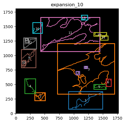
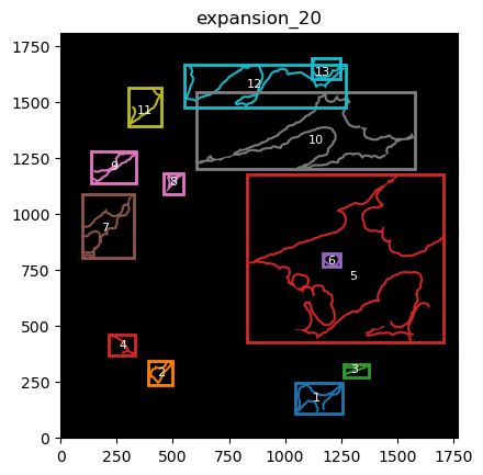
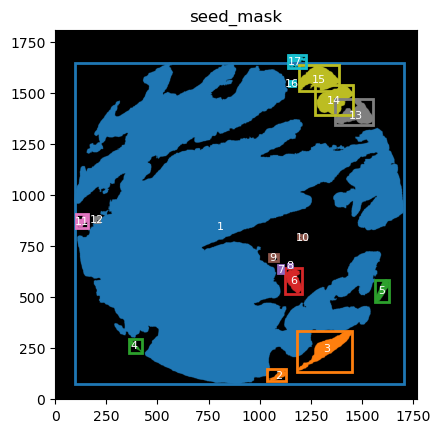
TA retrieves multiple mask dicts: * binary_expansions: with binary masks * labeled_expansions: with labelled object * referenced_objects: for hierarchy analysis

We can plot the masks simply just as with simple colors. There is also a function in GM to plot labelled masks with bounding boxes.

for mask in TA.labeled_expansions:
    labeled_mask = TA.labeled_expansions[mask]
    GM.plot_labeled_masks(label_mask=labeled_mask,
                       mask_name = mask, show=False)

you can now define the parameters that best suit the full cohort to define the contours and run for all files in the cohort.

Considerations:

probably set logger to write so a file with all the logging save to a report file ( get the file to a single core or do a single file for all the cohort is up to you) save the images and plots that may be necessary for the analysis later. Plotting and save takes time, but in some cases may be saving time to prevent you to redo analysis to obtain a figure.

How the same analysis look like using SOM.

Bin the image and aply a SOM cluster Each image is analysed separately

# Extract the filename without extension
filename = os.path.basename(file_csv).split('.')[0]

# Extract the desired part
name_file = '_'.join(filename.split('_')[:2])

We will get the bins defined in bin size from a list of df. In this case just one df of an image

These bins are not overlapping

The counts of eachbin with all the space information are saved in an adata object.

Preprocess bin applies single cell normalization oipeline to the bin information ( normalize total and log1) and filters out empty bins <10 counts.

bin_size = 5  # 10
min_counts = 10 # 10
unique_targets = df_total['target'].unique()

GB = GetBins(bin_size, unique_targets, logger)
GB.get_bin_cohort(df_list= [df_total], df_name_list = [name_file], cohort_name = 'HLA')
GB.preprocess_bin(min_counts = min_counts)
adata = GB.adata

2025-06-20 15:31:54,159 - contour_logger - INFO - Time to get bins for 1 dataframes: 1.93 seconds
2025-06-20 15:31:54,159 - contour_logger - INFO - Number of bins: 99374
2025-06-20 15:31:54,159 - contour_logger - INFO - Number of genes: 480

Now that we have the bins of the images. We can apply a SOM cluster. we will apply a SOM map with 2 cells, and see if it accurately divides tumour from stroma due to their big differences.

GC = GetContour(adata, logger)
GC.run_som(som_shape = (2,1), n_iter = 5000, sigma=.5, learning_rate=.5, random_state = 42)

2025-06-20 15:32:22,804 - contour_logger - INFO - Time to run som on 78461 bins: 0.93
2025-06-20 15:32:22,805 - contour_logger - INFO - Number of clusters: 2
2025-06-20 15:32:22,806 - contour_logger - INFO - number of bins in each cluster: cluster_som
0    42722
1    35739
Name: count, dtype: int64

As one can see this is almost instaneously. We can eval the differentially gene expression. one can use the GC.adata object and run preferred analysis. You can also use GC.eval_som_statistical

GC.eval_som_statistical(top_n=10)

2025-06-20 15:32:27,736 - contour_logger - INFO - n top genes for group 0
2025-06-20 15:32:27,738 - contour_logger - INFO - 
     names      scores  logfoldchanges  pvals  pvals_adj group
0    EPCAM  496.127167        4.710810    0.0        0.0     0
1    KRT18  401.328308        4.123829    0.0        0.0     0
2     LCN2  350.054199        4.303699    0.0        0.0     0
3     KRT8  204.175812        3.766609    0.0        0.0     0
4    CCL20  203.358932        3.733404    0.0        0.0     0
5      CA9  167.450836        4.739976    0.0        0.0     0
6    BIRC3  165.406113        3.378658    0.0        0.0     0
7    HLA-G  163.212875        1.587320    0.0        0.0     0
8   IFITM1  163.142197        2.525657    0.0        0.0     0
9  CEACAM1  161.894699        4.590243    0.0        0.0     0
2025-06-20 15:32:27,743 - contour_logger - INFO - n top genes for group 1
2025-06-20 15:32:27,745 - contour_logger - INFO - 
     names      scores  logfoldchanges  pvals  pvals_adj group
0    SPARC  367.663055        4.587291    0.0        0.0     1
1   COL1A1  347.223572        4.167460    0.0        0.0     1
2   IGFBP7  191.690048        4.526878    0.0        0.0     1
3      LUM  190.487732        4.909051    0.0        0.0     1
4    TIMP2  187.690933        4.334179    0.0        0.0     1
5   COL3A1  186.767471        5.427709    0.0        0.0     1
6      VIM  157.729630        2.898454    0.0        0.0     1
7  COL11A1  147.477905        5.134010    0.0        0.0     1
8   COL6A2  132.532669        4.741213    0.0        0.0     1
9    TAGLN  131.269485        4.528151    0.0        0.0     1

From the genes it appears that is separating bins based n stroma/ tumour .

Let’s see graphicaly

we can see in two different ways. one is to transform the bins into an image again using GC.get_som_2d_image(bin_size = 10) and plot it with GC.plot_som. 

The other option is to use squidpy and the centroids information stored in the adata object. In this one only the centroids are plotted ( but all the bins have the same size) 

import matplotlib.colors as mcolors
import squidpy as sq

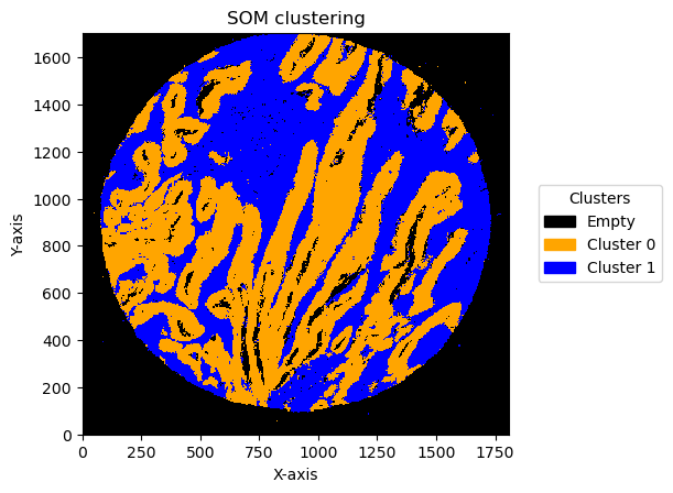
som_images = GC.get_som_2d_image(bin_size = 5)

# Create a custom colormap and legends 
cmap = mcolors.ListedColormap(['black', 'orange', 'blue',])
legend_labels = {0: 'Empty', 1: 'Cluster 0', 2: 'Cluster 1'}

for name, som_image in som_images.items():
    print(name)
    GC.plot_som(som_image, cmap = cmap, path=None, show=True, figsize=(5, 5), ax=None, legend_labels=legend_labels)

/home/martinha/miniconda3/envs/GRIDGEN/lib/python3.11/site-packages/dask/dataframe/__init__.py:31: FutureWarning: The legacy Dask DataFrame implementation is deprecated and will be removed in a future version. Set the configuration option `dataframe.query-planning` to `True` or None to enable the new Dask Dataframe implementation and silence this warning.
  warnings.warn(
/home/martinha/miniconda3/envs/GRIDGEN/lib/python3.11/site-packages/anndata/utils.py:434: FutureWarning: Importing read_text from `anndata` is deprecated. Import anndata.io.read_text instead.
  warnings.warn(msg, FutureWarning)

TMA1_Selection22

# adata.obsm["spatial"] = adata.obs[["x_centroid", "y_centroid"]].copy().to_numpy()
unique_cases =adata.obs['name'].unique()
for case in unique_cases:
    # Filter the AnnData object for the current case
    adata_case = adata[adata.obs['name'] == case, :]
    print(case)
    plt.rcParams["figure.figsize"] = (5, 4)
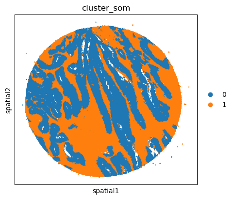
    sq.pl.spatial_scatter(
            adata_case,
            library_id='name',
            shape=None,
            color=["cluster_som"],
            size=1,
    )
    plt.show()

TMA1_Selection22

/home/martinha/miniconda3/envs/GRIDGEN/lib/python3.11/site-packages/scanpy/plotting/_utils.py:487: ImplicitModificationWarning: Trying to modify attribute `._uns` of view, initializing view as actual.
  adata.uns[value_to_plot + "_colors"] = colors_list
/home/martinha/miniconda3/envs/GRIDGEN/lib/python3.11/site-packages/squidpy/pl/_spatial_utils.py:976: UserWarning: No data for colormapping provided via 'c'. Parameters 'cmap', 'norm' will be ignored
  _cax = scatter(

We can use this information to build masks as we saw based on the contours defined by genes.

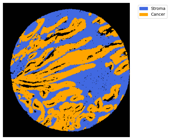
SOM clusters are numbered. one needs to identify the identity of these clusters. from GC.eval_som_statistical(top_n=10), we can see that cluster 0 is Stroma (SPARC, COL1A1, VIM … ) and 1 is tumour (EPCAM, KRT18, KRT8 …)

name, som_image = list(som_images.items())[0]
# pass the contour area threshold
GM = get_masks.GetMasks(image_shape = (som_image.shape[0], som_image.shape[1]))
mask_S = (som_image==2).astype(np.uint8) * 255
GM.mask_S = (GM.filter_binary_mask_by_area(mask_S, min_area=700))
mask_T = (som_image==1).astype(np.uint8) * 255
GM.mask_T = (GM.filter_binary_mask_by_area(mask_T, min_area=700))

GM.plot_masks(masks=[GM.mask_S, GM.mask_T], mask_names = ['Stroma', 'Cancer'],
          background_color=(1, 1, 1), 
              mask_colors={'Stroma': (65, 105, 225), 'Cancer': (255, 165, 0)},   # {'Stroma': (0, 0, 255), 'Tumour': (255, 0, 0)
              figsize= (6,6),
              path=None, show=True, ax=None)

2025-06-20 15:34:17,418 - gridgen.get_masks.GetMasks - INFO - Initialized GetMasks

With the masks, we can proceed and do the remaining pipeline with expansions, resuming mask information and hierarchy analysis as described in other notebooks. Important parameters include the bin size and the number of units in SOM (see appropriate notebook).

Effect of bin size and number of units

In this pipeline there are things that can change the result. One is the bin size and the second one is the number of units in SOM .

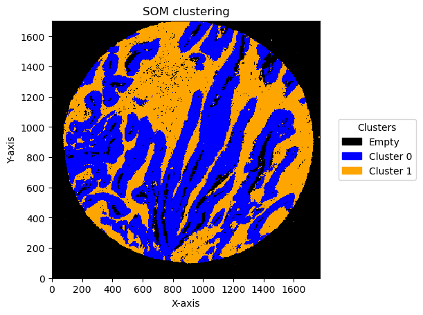
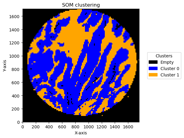
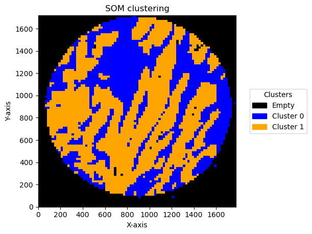
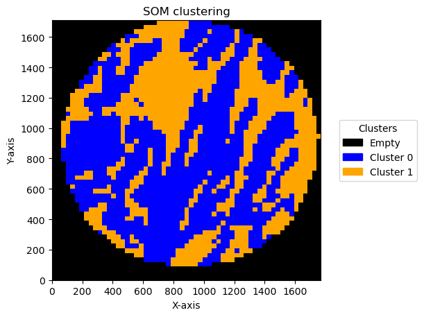
We can see the result effect of changing the bin size below:

cmap = mcolors.ListedColormap(['black', 'blue', 'orange'])
legend_labels = {0: 'Empty', 1: 'Cluster 0', 2: 'Cluster 1'}
plot_data = []

for bin_size in [5,10,15,20,30,50,70]:
    min_counts = bin_size *3 
    unique_targets = df_total['target'].unique()
    
    GB = GetBins(bin_size, unique_targets, logger)
    GB.get_bin_cohort(df_list= [df_total], df_name_list = [name_file], cohort_name = 'HLA')
    GB.preprocess_bin(min_counts = min_counts)
    adata = GB.adata
    GC = GetContour(adata, logger)
    GC.run_som(som_shape = (2,1), n_iter = 5000, sigma=.5, learning_rate=.5, random_state = 42)
    
    som_image = GC.get_som_2d_image(bin_size)
    plot_data.append((som_image, bin_size))

2025-06-20 15:35:37,545 - contour_logger - INFO - Time to get bins for 1 dataframes: 2.13 seconds
2025-06-20 15:35:37,546 - contour_logger - INFO - Number of bins: 99374
2025-06-20 15:35:37,546 - contour_logger - INFO - Number of genes: 480
2025-06-20 15:35:38,930 - contour_logger - INFO - Time to run som on 76725 bins: 0.93
2025-06-20 15:35:38,931 - contour_logger - INFO - Number of clusters: 2
2025-06-20 15:35:38,932 - contour_logger - INFO - number of bins in each cluster: cluster_som
0    41714
1    35011
Name: count, dtype: int64
2025-06-20 15:35:43,033 - contour_logger - INFO - Time to get bins for 1 dataframes: 1.44 seconds
2025-06-20 15:35:43,034 - contour_logger - INFO - Number of bins: 28640
2025-06-20 15:35:43,034 - contour_logger - INFO - Number of genes: 480
2025-06-20 15:35:43,525 - contour_logger - INFO - Time to run som on 20234 bins: 0.36
2025-06-20 15:35:43,526 - contour_logger - INFO - Number of clusters: 2
2025-06-20 15:35:43,527 - contour_logger - INFO - number of bins in each cluster: cluster_som
0    10871
1     9363
Name: count, dtype: int64
2025-06-20 15:35:45,627 - contour_logger - INFO - Time to get bins for 1 dataframes: 1.29 seconds
2025-06-20 15:35:45,628 - contour_logger - INFO - Number of bins: 13524
2025-06-20 15:35:45,628 - contour_logger - INFO - Number of genes: 480
2025-06-20 15:35:45,930 - contour_logger - INFO - Time to run som on 9196 bins: 0.24
2025-06-20 15:35:45,931 - contour_logger - INFO - Number of clusters: 2
2025-06-20 15:35:45,932 - contour_logger - INFO - number of bins in each cluster: cluster_som
0    5444
1    3752
Name: count, dtype: int64
2025-06-20 15:35:47,621 - contour_logger - INFO - Time to get bins for 1 dataframes: 1.24 seconds
2025-06-20 15:35:47,622 - contour_logger - INFO - Number of bins: 7842
2025-06-20 15:35:47,622 - contour_logger - INFO - Number of genes: 480
2025-06-20 15:35:47,858 - contour_logger - INFO - Time to run som on 5262 bins: 0.20
2025-06-20 15:35:47,858 - contour_logger - INFO - Number of clusters: 2
2025-06-20 15:35:47,859 - contour_logger - INFO - number of bins in each cluster: cluster_som
1    3084
0    2178
Name: count, dtype: int64
2025-06-20 15:35:49,269 - contour_logger - INFO - Time to get bins for 1 dataframes: 1.11 seconds
2025-06-20 15:35:49,270 - contour_logger - INFO - Number of bins: 3527
2025-06-20 15:35:49,270 - contour_logger - INFO - Number of genes: 480
2025-06-20 15:35:49,456 - contour_logger - INFO - Time to run som on 2390 bins: 0.17
2025-06-20 15:35:49,457 - contour_logger - INFO - Number of clusters: 2
2025-06-20 15:35:49,458 - contour_logger - INFO - number of bins in each cluster: cluster_som
0    1394
1     996
Name: count, dtype: int64
2025-06-20 15:35:50,779 - contour_logger - INFO - Time to get bins for 1 dataframes: 1.10 seconds
2025-06-20 15:35:50,779 - contour_logger - INFO - Number of bins: 1302
2025-06-20 15:35:50,779 - contour_logger - INFO - Number of genes: 480
2025-06-20 15:35:50,935 - contour_logger - INFO - Time to run som on 908 bins: 0.15
2025-06-20 15:35:50,935 - contour_logger - INFO - Number of clusters: 2
2025-06-20 15:35:50,936 - contour_logger - INFO - number of bins in each cluster: cluster_som
0    456
1    452
Name: count, dtype: int64
2025-06-20 15:35:52,176 - contour_logger - INFO - Time to get bins for 1 dataframes: 1.08 seconds
2025-06-20 15:35:52,177 - contour_logger - INFO - Number of bins: 664
2025-06-20 15:35:52,177 - contour_logger - INFO - Number of genes: 480
2025-06-20 15:35:52,331 - contour_logger - INFO - Time to run som on 490 bins: 0.15
2025-06-20 15:35:52,332 - contour_logger - INFO - Number of clusters: 2
2025-06-20 15:35:52,332 - contour_logger - INFO - number of bins in each cluster: cluster_som
1    328
0    162
Name: count, dtype: int64

for som_image, bin_size in plot_data:
    for name, image in som_image.items():
        print(f"Plotting bin size: {bin_size}, SOM name: {name}")
        GC.plot_som(image, cmap=cmap, path=None, show=True, figsize=(5, 5), ax=None, legend_labels=legend_labels)

Plotting bin size: 5, SOM name: TMA1_Selection22

Plotting bin size: 10, SOM name: TMA1_Selection22

Plotting bin size: 15, SOM name: TMA1_Selection22

Plotting bin size: 20, SOM name: TMA1_Selection22

Plotting bin size: 30, SOM name: TMA1_Selection22

Plotting bin size: 50, SOM name: TMA1_Selection22

Plotting bin size: 70, SOM name: TMA1_Selection22

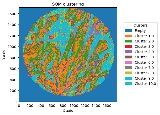
check how the number of units and distribution on the SOM map can reflect in the clusters obtained

cmap = mcolors.ListedColormap(['black', 'blue', 'orange'])
legend_labels = {0: 'Empty', 1: 'Cluster 0', 2: 'Cluster 1'}
plot_data = []

for som_size in [(2,1), (3,1), (2,2),(3,3), (5,2)]:
    bin_size = 10
    min_counts = 20 
    unique_targets = df_total['target'].unique()
    
    GB = GetBins(bin_size, unique_targets, logger)
    GB.get_bin_cohort(df_list= [df_total], df_name_list = [name_file], cohort_name = 'HLA')
    GB.preprocess_bin(min_counts = min_counts)
    adata = GB.adata
    GC = GetContour(adata, logger)
    GC.run_som(som_shape = som_size, n_iter = 5000, sigma=.5, learning_rate=.5, random_state = 42)
    
    som_image = GC.get_som_2d_image(bin_size)
    plot_data.append((som_image, bin_size))

2025-06-20 15:36:47,109 - contour_logger - INFO - Time to get bins for 1 dataframes: 1.39 seconds
2025-06-20 15:36:47,109 - contour_logger - INFO - Number of bins: 28640
2025-06-20 15:36:47,109 - contour_logger - INFO - Number of genes: 480
2025-06-20 15:36:47,593 - contour_logger - INFO - Time to run som on 20450 bins: 0.35
2025-06-20 15:36:47,593 - contour_logger - INFO - Number of clusters: 2
2025-06-20 15:36:47,594 - contour_logger - INFO - number of bins in each cluster: cluster_som
0    11561
1     8889
Name: count, dtype: int64
2025-06-20 15:36:49,934 - contour_logger - INFO - Time to get bins for 1 dataframes: 1.52 seconds
2025-06-20 15:36:49,934 - contour_logger - INFO - Number of bins: 28640
2025-06-20 15:36:49,934 - contour_logger - INFO - Number of genes: 480
2025-06-20 15:36:50,432 - contour_logger - INFO - Time to run som on 20450 bins: 0.36
2025-06-20 15:36:50,432 - contour_logger - INFO - Number of clusters: 3
2025-06-20 15:36:50,433 - contour_logger - INFO - number of bins in each cluster: cluster_som
2    10064
0     7324
1     3062
Name: count, dtype: int64
2025-06-20 15:36:52,663 - contour_logger - INFO - Time to get bins for 1 dataframes: 1.41 seconds
2025-06-20 15:36:52,663 - contour_logger - INFO - Number of bins: 28640
2025-06-20 15:36:52,663 - contour_logger - INFO - Number of genes: 480
2025-06-20 15:36:53,195 - contour_logger - INFO - Time to run som on 20450 bins: 0.40
2025-06-20 15:36:53,195 - contour_logger - INFO - Number of clusters: 4
2025-06-20 15:36:53,196 - contour_logger - INFO - number of bins in each cluster: cluster_som
1    9425
2    5733
0    3013
3    2279
Name: count, dtype: int64
2025-06-20 15:36:55,468 - contour_logger - INFO - Time to get bins for 1 dataframes: 1.45 seconds
2025-06-20 15:36:55,469 - contour_logger - INFO - Number of bins: 28640
2025-06-20 15:36:55,469 - contour_logger - INFO - Number of genes: 480
2025-06-20 15:36:56,088 - contour_logger - INFO - Time to run som on 20450 bins: 0.49
2025-06-20 15:36:56,089 - contour_logger - INFO - Number of clusters: 9
2025-06-20 15:36:56,090 - contour_logger - INFO - number of bins in each cluster: cluster_som
6    4778
5    4740
8    3730
3    1867
4    1249
2    1225
0    1176
1    1108
7     577
Name: count, dtype: int64
2025-06-20 15:36:58,350 - contour_logger - INFO - Time to get bins for 1 dataframes: 1.44 seconds
2025-06-20 15:36:58,351 - contour_logger - INFO - Number of bins: 28640
2025-06-20 15:36:58,351 - contour_logger - INFO - Number of genes: 480
2025-06-20 15:36:58,985 - contour_logger - INFO - Time to run som on 20450 bins: 0.50
2025-06-20 15:36:58,985 - contour_logger - INFO - Number of clusters: 10
2025-06-20 15:36:58,986 - contour_logger - INFO - number of bins in each cluster: cluster_som
9    4708
0    4478
1    4189
7    1787
2    1548
6    1067
4    1032
3     612
8     516
5     513
Name: count, dtype: int64

for som_image, bin_size in plot_data:
    for name, image in som_image.items():
        # Get unique clusters from your data (e.g., via np.unique(cluster_data))
        unique_clusters = np.unique(image)
        
        # Create the legend_labels dictionary only for detected clusters
        legend_labels = {i: f'Cluster {i}' for i in unique_clusters}
        
        # Optional: set specific labels if certain clusters have special meanings
        if 0 in unique_clusters:
            legend_labels[0] = 'Empty'
        print(f"Plotting bin size: {bin_size}, SOM name: {name}")
        GC.plot_som(image, cmap=plt.cm.tab10, path=None, show=True, figsize=(5, 5), ax=None, legend_labels=legend_labels)

Plotting bin size: 10, SOM name: TMA1_Selection22

Plotting bin size: 10, SOM name: TMA1_Selection22

Plotting bin size: 10, SOM name: TMA1_Selection22

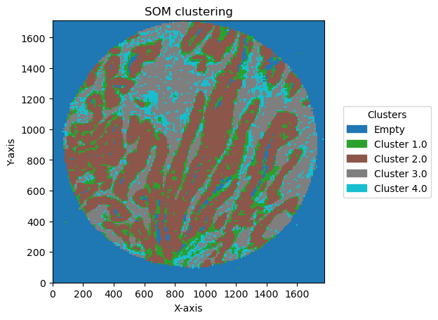
Plotting bin size: 10, SOM name: TMA1_Selection22

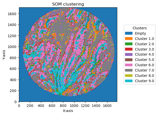
Plotting bin size: 10, SOM name: TMA1_Selection22